Nd787 C5 L3 A07 L Linearized Model V3

Linearization

We've been using the following for our state vector:

\mathbf{x} = \begin{bmatrix} x_I\\ z_I\\ \theta \\ u \\ w \\ q \end{bmatrix}

And the non-linear equations of motion are:

\begin{aligned} \dot{x}_I &= u \cos \theta + w \sin \theta \\ \dot{z}_I &= -u \sin \theta + w \cos \theta \\ \dot{\theta} &= q \\ \dot{u} &=- qw \\ \dot{w} &= qu \\ \dot{q} &= 0 \\ \end{aligned}

We can write these equations more concisely and generally as some function of the current state and the controls:

\dot{x} = f(x, u)

We define a trim state x^ (and associated trim state controls u^) and a deviation from trim \bar{x} such that

\bar{x} = x - x^*

This means that

\begin{aligned} \dot{\bar{x}} &= \dot{x} - \dot{x}^* \\ &= f(x,u) - f(x^*, u^*) \\ &= f(x^* + \bar{x}, u^* + \bar{u}) - f(x^*, u^*) \end{aligned}

Taking a Taylor series expansion, we can write this as

\dot{\bar{x}} =f(x^*, u^*) + \frac{\partial f(x^*, u^*)}{\partial x} \bar{x} + \frac{\partial f(x^*, u^*)}{\partial u} \bar{u} + \ldots - f(x^*, u^*)

Where I've used \ldots to represent higher order terms in the Taylor expansion. Dropping these terms and canceling out the trim state, we find

\dot{\bar{x}} \approx \frac{\partial f(x^*, u^*)}{\partial x} \bar{x} + \frac{\partial f(x^*, u^*)}{\partial u} \bar{u}

Linearized Equations

It winds up being convenient to remove w from the state vector and replace it with the angle of attack \alpha. These variables are related:

\begin{aligned} w &= V \sin\alpha \\ \bar{w} &= V^* \cos \alpha^* \bar{\alpha} \end{aligned}

When we work out the Jacobians of the resulting state vector, we get the following linearized equations of motion:

\begin{aligned} \begin{bmatrix} \dot{\bar{x_I}} \\ \dot{\bar{z_I}} \\ \dot{\bar{\theta}} \\ \dot{\bar{u}} \\ \dot{\bar{\alpha}} \\ \dot{\bar{q}} \end{bmatrix} &= \begin{bmatrix} 0 & 0 & -u^* \sin \theta^* + w^* \cos \theta^* & \cos \theta^* & V^*\sin \theta^* \cos \alpha^* & 0 \\ 0 & 0 & -u^* \cos \theta^* - w^* \sin \theta^* & -\sin \theta^* & V^* \cos \theta^* \cos \alpha^*& 0 \\ 0 & 0 & 0 & 0 & 0 & 1 \\ 0 & 0 & -g\cos\theta^* & X_u & X_w V^* \cos\alpha & X_q \\ 0 & 0 & \frac{-g\sin\theta^*}{V^* \cos \alpha^*} & \frac{Z_u}{V^* \cos \alpha^*} & Z_w & \frac{Z_q}{V^* \cos \alpha^*} \\ 0 & 0 & 0 & M_u & M_w V^* \cos \alpha^* & M_q \end{bmatrix} \cdot \begin{bmatrix} \bar{x_I} \\ \bar{z_I} \\ \bar{\theta} \\ \bar{u} \\ \bar{\alpha} \\ \bar{q} \end{bmatrix} \\ &+ \begin{bmatrix} 0 & 0 & \\ 0 & 0 & \\ 0 & 0 & \\ X_{\delta e} & X_{\delta t} \\ \frac{Z_{\delta e}}{V \cos \alpha} & 0 \\ M_{\delta e} & 0 \end{bmatrix} \cdot \begin{bmatrix} \bar{\delta e}\\ \bar{\delta T} \end{bmatrix} \end{aligned}

The 6 \times 6 matrix on the first line is the stability matrix. The 6 \times 2 matrix on the second line is the control-effect matrix.

Note that we've introduced some new coefficients in order to write these more compactly.

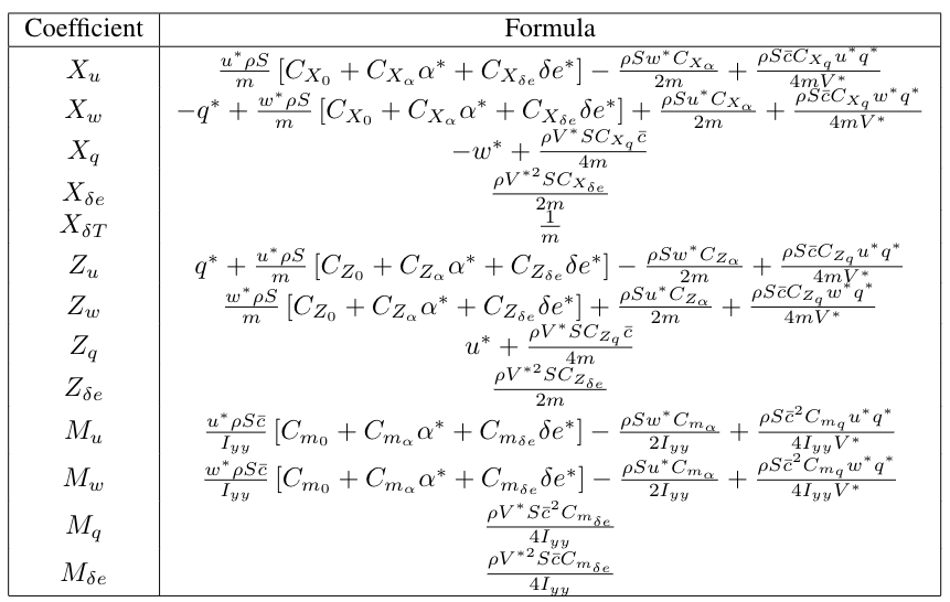
Remember: you can find all of these equations in the fixed wing cheat sheet.

Next Concept